Introduction to BNs
Bayesian networks have been successfully applied to create consistent probabilistic representations of uncertain knowledge in diverse fields such as medical diagnosis (Spiegelhalter et al., 1989), image recognition (Booker & Hota, 1986), language understanding (Charniak & Goldman, 1989a, 1989b), search algorithms (Hansson & Mayer, 1989), and many others. Heckerman et. al. (1995b) provides a detailed list of recent applications of Bayesian Networks.
One of the most important features of Bayesian networks is the fact that they provide an elegant mathematical structure for modeling complicated relationships among random variables while keeping a relatively simple visualization of these relationships. The figure below gives three simple examples of qualitatively different probability relationships among three random variables.
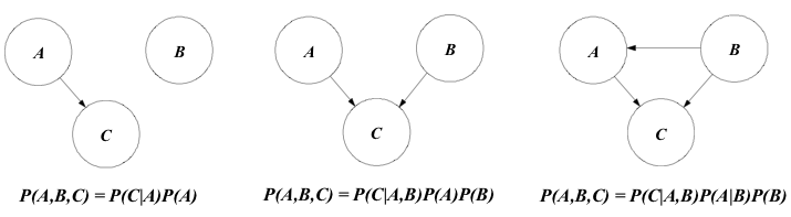
As a means for realizing the communication power of this representation, one could compare two hypothetical scenarios in which a domain expert with little background in probability tries to interpret what is represented in the figure above. Initially, suppose that she is allowed to look only to the written equations below the pictures. In this case, we believe that she will have to think at least twice before making any conclusion on the relationships among events A, B, and C. On the other hand, if she is allowed to look only to the pictures, it seems fair to say that she will immediately perceive that in the leftmost picture, for example, event B is independent of events A and C, and event C depends on event A. Also, simply comparing the pictures would allow her to see that, in the center picture, A is now dependent on B, and that in the rightmost picture B influences both A and C. Advantages of easily interpretable graphical representation become more apparent as the number of hypothesis and the complexity of the problem increases.
Pearl's Bi-directional Belief Updating Algorithm
One of the most powerful characteristics of Bayesian Networks is its ability to update the beliefs of each random variable via bi-directional propagation of new information through the whole structure. This was initially achieved by an algorithm proposed by Pearl (1988) that fuses and propagates the impact of new evidence providing each node with a belief vector consistent with the axioms of probability theory. The figure below shows a graphical representation of Pearl's bi-directional propagation scheme.
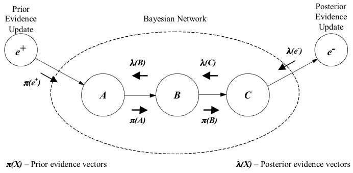
Roughly speaking, information can be inserted in Bayesian Networks through a data updating in the prior probabilities or in the posterior probabilities. In the first case,the new data will flow via a π row vector (prior evidence vector), while in the former case data will flow via a λ column vector (posterior evidence vector). Both vectors update the node belief (say node B) by the equation:
![]()
where “α” is a normalizing constant, and “ • “ means term by term multiplication (inner or dot product). The resulting column vector is the new belief of node B, clearly, vector Bel(B) will have as many elements as the number of states of the random variable depicted by node B.
Nodes of a Bayesian network have different number of states, which will reflect in the number of elements each π or λ vectors will have. After receiving a π vector with updated information from a parent node (say A), node B will send its own π vector to its children nodes. The equation used in node B for creating its π vector is:
![]()
where “ ⊗ “ means vector multiplication (or congruent product), and MB|A is the likelihood matrix, or conditional probability distribution matrix between nodes B and A.
When receiving a λ vector with updated information from a child node (say node C), node B will send its own λ vector to its parent nodes. The formula used in node B for creating its λ vector is:
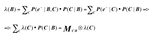
where the resulting column vector λ(B) is then transmitted to parent nodes.
However, a node usually has multiple children, which means it may receive different λ vectors. The node internal algorithm must be able to deal with these vectors concurrently, as more than one node can send λ vectors at the same time. The figure below shows the internal structure of a single node processor, which explains how this problem was solved by Pearl's algorithm. In fact, the graph itself is an adaptation of the one used in page 168 of Pearl's book (Pearl, 1988).
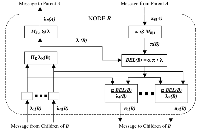
As an example illustrating the effectiveness of the algorithm, let's imagine the case in which node B has two children (say nodes C and D). When a λ vector is received from node C, that information will update node B's belief vector and this new belief vector will be sent to parent nodes (as λ vectors), and to children nodes (as π vectors). However, sending a π vector back to node C would generate a new update in node C with the same data it sent before, thus creating a loop. The division that happens in the lower left part of the diagram prevents this unwanted characteristic. The message that is sent to children nodes is BEL(B) divided by the respective children node λ vector, eliminating the possibility of double counting the information. In our example, node D will receive a π vector from node B that has the information sent by node C (which means that node C's new information is propagated to D). In contrast, node C will receive a π vector that is divided by λC so the information already sent will not be double counted.
Other Belief Updating Algorithms for Bayesian Networks
Pearl’s algorithm performs exact Bayesian updating, but only for singly connected networks. Subsequently, general Bayesian updating algorithms have been developed. One of the most commonly applied is the Junction Tree algorithm (Lauritzen & Spiegelhalter, 1988). Neapolitan (2003) provides a discussion on many Bayesian propagation algorithms. Although Cooper (1987) showed that exact belief propagation in Bayesian Networks can be NP-Hard, exact computation is practical for many problems of practical interest.
Some complex applications are too challenging for exact inference, and require approximate solutions (Dagum & Luby, 1993). Many computationally efficient inference algorithms have been developed, such as probabilistic logic sampling (Henrion, 1988), likelihood weighting (Fung & Chang, 1989; Shachter & Peot, 1990), backward sampling (Fung & del Favero, 1994), Adaptive Importance Sampling (Cheng & Druzdzel, 2000), and Approximate Posterior Importance Sampling (Druzdzel & Yuan, 2003).
Those algorithms allow the impact of evidence about one node to propagate to other nodes in multiply-connected trees, making Bayesian Networks a reliable engine for probabilistic inference. The prospective reader will find comprehensive coverage of Bayesian Networks in a large and growing literature on this subject, such as Pearl (1988), Neapolitan (1990, 2003), Oliver & Smith (1990), Charniak (1991), Jensen (1996, 2001), or Korb & Nicholson (2003).
Limitations of Probabilistic Reasoning with Bayesian Networks
Bayesian Networks have received praise for being a powerful tool for performing probabilistic inference, but they do have some limitations that impede their application to complex problems. As the technique grew in popularity, Bayesian Network's limitations became increasingly apparent. One of the most important limitations for it to be applied in the context of PR-OWL is the fact that, although a powerful tool, BNs are not expressive enough for many real-world applications. More specifically, Bayesian Networks assume a simple attribute-value representation – that is, each problem instance involves reasoning about the same fixed number of attributes, with only the evidence values changing from problem instance to problem instance.
This type of representation is inadequate for many problems of practical importance. Many domains require reasoning about varying numbers of related entities of different types, where the numbers, types and relationships among entities usually cannot be specified in advance and may have uncertainty in their own definitions. As will be demonstrated below, Bayesian networks are insufficiently expressive for such problems.
The (Basic) Starship Case Study
Choosing a particular real-life domain would pose the risk of getting bogged down in domain-specific detail. For this reason, we opted to construct a case study based on the popular television series Star Trek. Nonetheless, the examples presented here have been constructed to be accessible to anyone having some familiarity with space-based science fiction. We begin our exposition narrating a highly simplified problem of detecting enemy starships.
In this simplified version of the PR-OWL Starship case study, the main task of a decision system is to model the problem of detecting Romulan starships (here considered as hostile by the United Federation of Planets) and assessing the level of danger they bring to our own starship, the Enterprise. All other starships are considered either friendly or neutral. Starship detection is performed by the Enterprise’s suite of sensors, which can correctly detect and discriminate starships with an accuracy of 95%. However, Romulan starships may be in “cloak mode,” which makes them invisible to the Enterprise’s sensors. Even for the most current sensor technology, the only hint of a nearby starship in cloak mode is a slight magnetic disturbance caused by the enormous amount of energy required for cloaking. The Enterprise has a magnetic disturbance sensor, but it is very hard to distinguish background magnetic disturbance from that generated by a nearby starship in cloak mode.
 This simplified situation is modeled by the BN depicted on the right (1), which also considers the characteristics of the zone of space where the action takes place. Each node in our BN has a finite number of mutually exclusive, collectively exhaustive states. The node Zone Nature (ZN) is a root node, and its prior probability distribution can be read directly from the BN (e.g. 80% for deep space). The probability distribution for Magnetic Disturbance Report (MDR) depends on the values of its parents ZN and Cloak Mode (CM). The strength of this influence is quantified via the conditional probability table (CPT) for node MDR, shown below. Similarly, Operator Species (OS) depends on ZN, and the two report nodes depend on CM and the hypothesis on which they are reporting.
Graphical models provide a powerful modeling framework and have been applied to many real world problems involving uncertainty. Yet, the model depicted above is of little use in a “real life” starship environment. After all, hostile starships cannot be expected to approach Enterprise one at a time so as to render its simple BN model usable. If four starships were closing in on the Enterprise, the BN depicted above would have to be replaced by the one shown below.
Unfortunately, building a BN for each possible number of nearby starships is not only a daunting task but also a pointless one, since there is no way of knowing in advance how many starships the Enterprise is going to encounter and thus which BN to use at any given time. In short, BNs lack the expressive power to represent entity types (e.g., starships) that can be instantiated as many times as required for the situation at hand.
In spite of its naiveté, we will briefly hold on to the premise that only one starship can be approaching the Enterprise at a time, so that the first BN presented here is valid. Furthermore, we will assume that the Enterprise is traveling in deep space, and its sensor reports imply that there is no trace of any nearby starship (i.e. the state of node SR state is Nothing). Further, there’s a newly arrived report indicating a strong magnetic disturbance (i.e. the state of node MDR is High). A brief look at the MDR node's CPT shows that the likelihood ratio for a high MDR is 7/5 = 1.4 in favor of a starship in cloak mode. Although this favors a cloaked starship in the vicinity, the evidence is not overwhelming.
Repetition is a powerful way to boost the discriminatory power of weak signals. As an example from airport terminal radars, a single pulse reflected from an aircraft usually arrives back to the radar receiver very weakened, making it hard to set apart from background noise. However, a steady sequence of reflected radar pulses is easily distinguishable from background noise.
Following the same logic, it is reasonable to assume that an abnormal background disturbance will show random fluctuation, whereas a disturbance caused by a starship in cloak mode would show a characteristic temporal pattern. Thus, when there is a cloaked starship nearby, the MDR state at any time depends on its previous state. A BN similar to the one below could capitalize on this for pattern recognition purposes.
Dynamic Bayesian Networks (DBNs) allow nodes to be repeated over time (Murphy, 1998). The BN shown here has both static and dynamic nodes, and thus is a partially dynamic Bayesian network (PDBN), also known as a temporal Bayesian network (Takikawa et al., 2002). While DBNs and PDBNs are useful for temporal recursion, a more general recursion capability is needed, as well as a parsimonious syntax for expressing recursive relationships.
What has been discussed here is just a glimpse of the issues that confront an engineer attempting to apply Bayesian networks to realistically complex problems. We did not provide a comprehensive analysis of the limitations of Bayesian networks for solving complex problems, since this brief overview is enough for making the point that even relatively simple situations might require more expressiveness than BNs can provide.
A much more powerful representational formalism is offered by first-order logic (FOL), which has the ability to represent entities of different types interacting with each other in varied ways. Sowa states that first-order logic “has enough expressive power to define all of mathematics, every digital computer that has ever been built, and the semantics of every version of logic, including itself” (Sowa, 2000, page 41). For this reason, FOL has become the de facto standard for logical systems from both a theoretical and practical standpoint.
However, systems based on classical first-order logic lack a theoretically principled, widely accepted, logically coherent methodology for reasoning under uncertainty. PR-OWL aims to fill this gap, as it merges the representational power of FOL with the elegant reasoning framework of Bayesian inference.